Distict level dynasticism

We calculate the the dynasty scor eof district by calcuating the years ruled by dynast in a district from 1974 to 2017.

district_name	dyn_prop
etawah	0.30
moradabad	0.24
mainpuri	0.23
azamgarh	0.22
muzaffarnagar	0.21
etah	0.21
mathura	0.21
lalitpur	0.20
saharanpur	0.19
shahjahanpur	0.18
hardoi	0.18
sitapur	0.17
gonda	0.17
baharaich	0.16
mirzapur	0.16
lucknow	0.16
rampur	0.15
budaun	0.15
pilibhit	0.14
mau	0.14
amethi	0.14
kasganj	0.14
chandauli	0.13
shamli	0.12
bareilly	0.12
varanasi	0.12
aligarh	0.11
firozabad	0.11
hathras	0.10
pratapgarh	0.10
farrukhabad	0.10
kannauj	0.10
mahoba	0.10
banda	0.10
deoria	0.10
ghaziabad	0.10
meerut	0.09
ghazipur	0.09
ambedkar nagar	0.09
gorakhpur	0.08
barabanki	0.08
kanpur nagar	0.08
faizabad	0.08
balrampur	0.08
kushi nagar	0.08
maharajganj	0.08
gautam buddha nagar	0.08
sambhal	0.07
agra	0.07
siddharth nagar	0.07
kheri	0.06
sultanpur	0.06
balia	0.06
unnao	0.05
allahabad	0.05
bulandsahar	0.04
bijnor	0.04
kaushambi	0.04
rae bareli	0.04
jaunpur	0.04
baghpat	0.03
basti	0.02
jhansi	0.02
amroha	0.00
hapur	0.00
shravasti	0.00
sant kabir nagar	0.00
auraiya	0.00
kanpur dehat	0.00
jalaun	0.00
hamirpur	0.00
bhadohi	0.00
chitrakoot	0.00
fatehpur	0.00
sonbhadra	0.00

census data

Das gupta

Question: In what kind of places do dynasticism arise ?

We use Aditya Das Gupta’s agricultural data which is available from 1957 to 1985. The mean of the relevant variables are plotted against years ruled by dynast those respective districts in the following scatter plot.

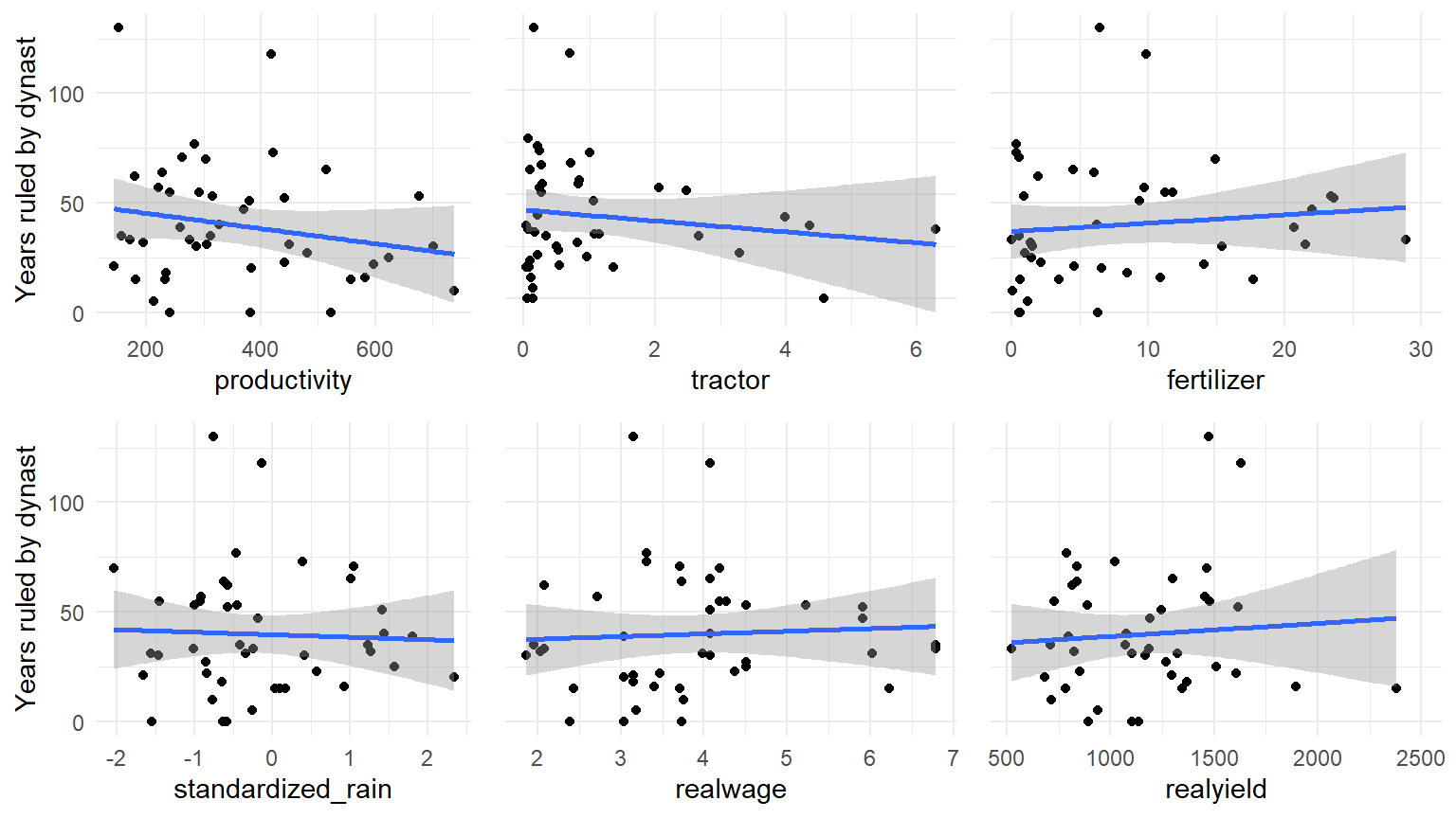
We take the mean of all the available variables and regress it against the number of years ruled by dynast in a district.


	Dependent variable:

	Dynast rule

mean_rain	-0.136
	(0.139)
mean_fertilizer	-0.031^***
	(0.006)
mean_prod	-0.003^***
	(0.0003)
mean_wage	0.181^***
	(0.029)
mean_tractor	-0.027
	(0.020)
mean_yield	0.001^***
	(0.0001)
Constant	3.554^***
	(0.140)

Observations	44
Log Likelihood	-467.404
Akaike Inf. Crit.	948.809

Note:	p<0.1; p<0.05; p<0.01

Dasgupta

Alexander

Alexander Lee’s state capacity data is available for the years 1964-1984. Just like we did in Dasgupta data, we take the mean of all the variables for our analysis and match it with the districts in our data. The two relevant variables are police and tax. The scatterplot shows those two variables relationship with the dynast rule - which is calculated as the sum of years ruled by dynasts in that particular districts.

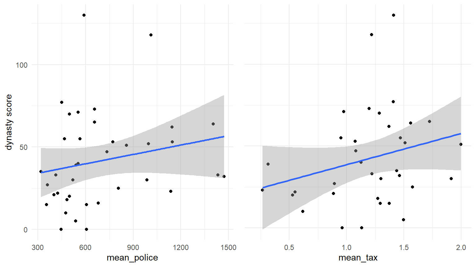
Here we regress the variables from both Das gupta and Lee’s data against the dynast rule.


	Dependent variable:

	Dynast rule

mean_rain	-0.011
	(0.141)
mean_fertilizer	-0.040^***
	(0.007)
mean_prod	-0.004^***
	(0.0004)
mean_wage	0.207^***
	(0.035)
mean_tractor	-0.015
	(0.024)
mean_yield	0.001^***
	(0.0001)
mean_police	0.001^***
	(0.0001)
mean_tax	-0.249^***
	(0.053)
Constant	3.475^***
	(0.160)

Observations	38
Log Likelihood	-378.903
Akaike Inf. Crit.	775.807

Note:	p<0.1; p<0.05; p<0.01

Dasgupta

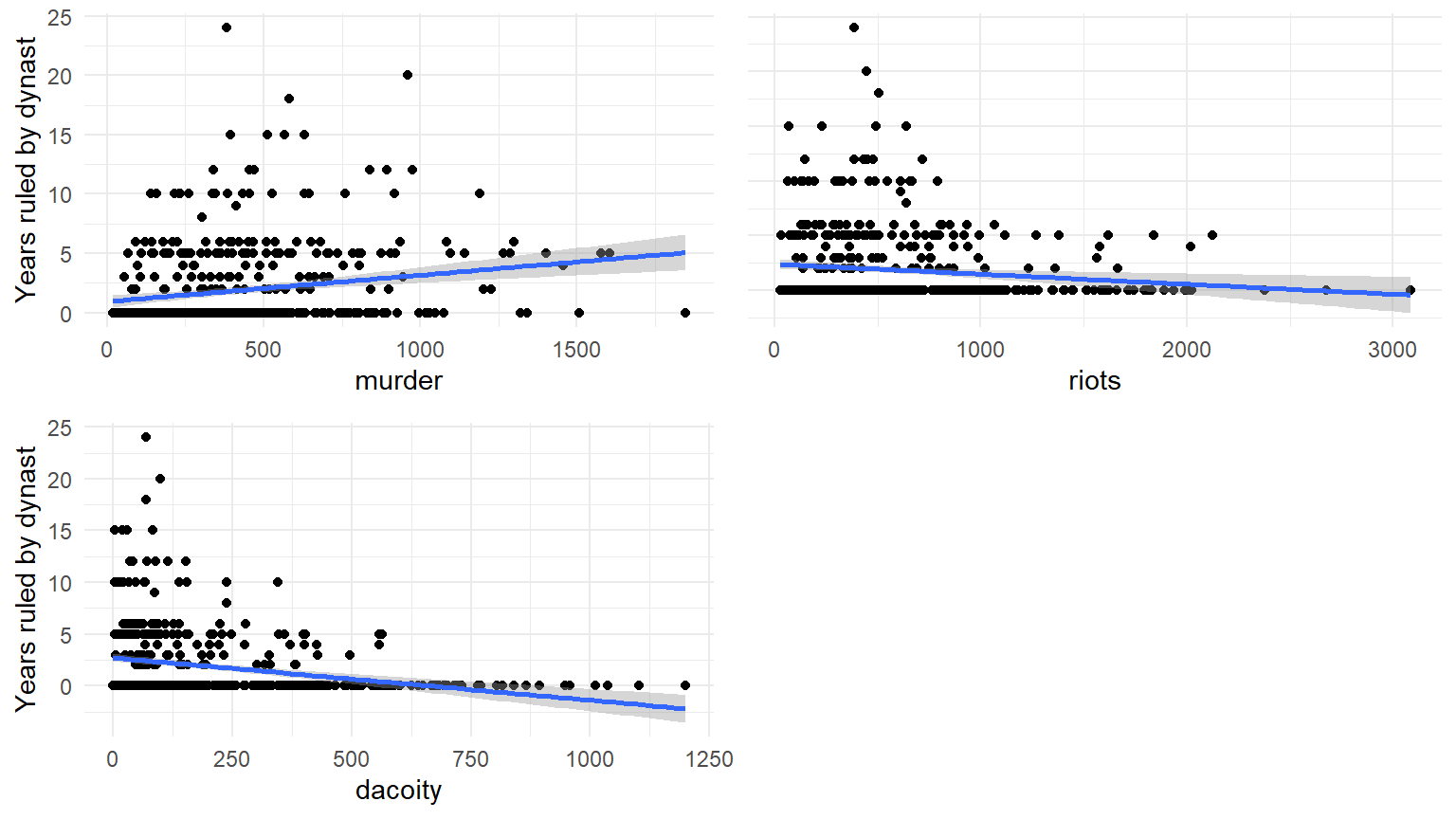
criminality

We use district level criminality data which is available since 1974 to to see how dynast rule and the criminal rates in a districts are correlated. First we run a scatter plot to see the direction and a poisson regression.


	Dependent variable:

	Dynast rule

dacoity	-0.003^***
	(0.001)

murder	0.001^***
	(0.0001)

riots	0.0005^***
	(0.0001)

factor(year)1977	15.330
	(297.908)

factor(year)1980	16.322
	(297.908)

factor(year)1985	15.626
	(297.908)

factor(year)1989	15.084
	(297.908)

factor(year)1991	15.098
	(297.908)

factor(year)1993	15.647
	(297.908)

factor(year)1996	16.747
	(297.908)

factor(year)2002	16.443
	(297.908)

factor(year)2007	16.786
	(297.908)

Constant	-15.655
	(297.908)


Observations	506
Log Likelihood	-1,113.533
Akaike Inf. Crit.	2,253.067

Note:	p<0.1; p<0.05; p<0.01